Not so long ago, linear diffusion was one of the process to be applied in many Computer Vision algorithms like feature detection, matching, etc. Now, a newer technique, known as Perona-Malik or non-linear diffusion, has arrived on the scene. Despite this, linear diffusion is still important due to its simplicity and ease of implementation. Further, the advantages of non-linear diffusion can only be appreciated if we have gone through linear diffusion first. So, before we begin, we will look at the process of diffusion as such.

Linear Diffusion

Let’s recall from our school days a process known as ‘diffusion’ in Physics where fluid or molecules move from higher concentration to lower concentration. In the same way, in Computer Vision, diffusion means pixel intensities move from a higher intensity region to lower intensity region. In linear diffusion, the rate of diffusion depends only on gradient (rate of change of pixel intensities at a given point) irrespective of pixel coordinates. Hence, the process is also known as isotropic diffusion. We’ll next look at a code implementing the same.

Matlab Implementation

In order to enable diffusion in an image, we’ve to apply a direction invariant filter to it. Usually, a Gaussian filter is a better option. Hence, linear diffusion is also known as Gaussian diffusion. A Matlab code implementing the filtering process is as follows:

function imgblr = linear_gaussian_diffusion(img, kernelsize, sigma)
% sigma is the standard deviation of the Gaussian filter
gs_kernal = fspecial('gaussian', kernelsize, sigma);

imgblr = imfilter(img, gs_kernal, 'replicate');

The function ‘imfilter’ does zero padding by default while applying a filter at the boundaries of the image. This may lead to high diffusion due to sudden changes at boundaries. In order to avoid the same, I’ve used an option ‘replicate’ which copies the value for a pixel outside the image from the nearest pixel.

Test Code

I’ll now use the above implemented function to perform diffusion on an image. The code used for testing is as follows:-

function res = test_linear_diffusion()
img0 = imread('mri1.jpg');
img0 = double(img0);
img0 = img0 - min(img0(:));
img0 = img0/max(img0(:));

img1 = linear_gaussian_diffusion(img0,31,1);

img2 = linear_gaussian_diffusion(img0,31,2);

img4 = linear_gaussian_diffusion(img0,31,4);

img8 = linear_gaussian_diffusion(img0,31,8);

img16 = linear_gaussian_diffusion(img0,31,16);

figure; title('Linear difusion');
subplot(2,3,1), imshow(img0,[]), title('original image');
subplot(2,3,2), imshow(img1,[]), title('kernel size = 31,sigma = 1');
subplot(2,3,3), imshow(img2,[]), title('kernel size = 31,sigma = 2');
subplot(2,3,4), imshow(img4,[]), title('kernel size = 31,sigma = 4');
subplot(2,3,5), imshow(img8,[]), title('kernel size = 31,sigma = 8');
subplot(2,3,6), imshow(img16,[]), title('kernel size = 31,sigma = 16');

res = true;

Though we can apply Gaussian diffusion on any image, I’ve observed that converting an image to double format with full contrast gives better result. The reasons are not hard to decipher. Double format has more range than integer format in Matlab. Further, stretching the pixel intensities to extreme ends ensure faster diffusion.

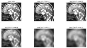
The above result points that the finer details are the first to vanish as a result of diffusion. The edges present in the image also get blurred, and diffusion creates homogeneous regions with coarse details.

Choice of Gaussian Filter

In order to apply linear diffusion, we have to first choose a Gaussian filter. There are two parameters here to decide—variance and filter size. We will discuss their effect on diffusion one by one in detail.

Variance of Gaussian Filter

The diffusion process is greatly affected by the variance of the Gaussian filter. Generally, higher the variance, higher is the rate of diffusion. As an example, the outcomes of diffusion for two variance values are shown below.

However, we will see soon one situation where increase in the variance doesn’t result in change in the rate of diffusion.

Size of Gaussian Filter

The kernel size of a Gaussian filter can be even or odd. However, an odd size Gaussian filter has an advantage that there is a single peak value which is not the case with an even size filter. For example, the below snippet provides the Gaussian filter values for an even and odd value. We can observe that the number of peaks is one in case of the odd value while it is 4 in case of the even value. Hence, usually an even size Gaussian filter is used for diffusion.

>> fspecial('gaussian', 3, 1)

ans =

0.0751 0.1238 0.0751
0.1238 0.2042 0.1238
0.0751 0.1238 0.0751

>> fspecial('gaussian', 4, 1)

ans =

0.0181 0.0492 0.0492 0.0181
0.0492 0.1336 0.1336 0.0492
0.0492 0.1336 0.1336 0.0492
0.0181 0.0492 0.0492 0.0181

The kernel size of a filter defines the region which will influence a pixel value on the application of the filter. In order to better understand the relation between the kernel size and the rate of diffusion, consider the result of diffusion for two different filter sizes.

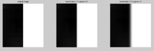
As can be seen, the diffusion is higher for larger size filter. However, it is also observed that after a certain point, the rate of diffusion has negligible increase with increase in kernel size.

Normalization of Gaussian Filter

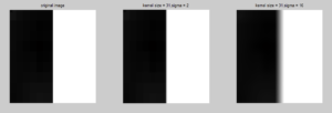
We have seen that diffusion depends on both variance and filter size. However, are the variance and filter size independent of each other? In order to seek answer of this question, consider the result of diffusion, as shown below, for two variance values.

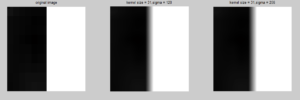
We can observe that there is negligible increase in diffusion despite doubling of sigma value (standard deviation). This is due to an important property of the discretized Gaussian filters obtained through Matlab. The Matlab implementation of the filter has normalized values i.e. the sum of the values is one. An example of the same is as follows:

gs_kernal = fspecial('gaussian', 7, 1000)

gs_kernal =

0.0204 0.0204 0.0204 0.0204 0.0204 0.0204 0.0204
0.0204 0.0204 0.0204 0.0204 0.0204 0.0204 0.0204
0.0204 0.0204 0.0204 0.0204 0.0204 0.0204 0.0204
0.0204 0.0204 0.0204 0.0204 0.0204 0.0204 0.0204
0.0204 0.0204 0.0204 0.0204 0.0204 0.0204 0.0204
0.0204 0.0204 0.0204 0.0204 0.0204 0.0204 0.0204
0.0204 0.0204 0.0204 0.0204 0.0204 0.0204 0.0204

sum(sum(gs_kernal))

ans =

1.0000

One consequence of the above property is that if we increase the sigma value of a Gaussian filter beyond a certain point, the filter starts behaving like an averaging filter with hardly any change in its values. In order to avoid the situation, we’ve to choose the kernel size in proportion the the sigma value. As per this article, a discrete filter of size six times the sigma value is a sufficient approximation for the Gaussian function, with same sigma, at every point on an image. This is the reason for negligible increase in diffusion with increase in the kernel size beyond a certain point.

Thus, we have only one parameter —variance—to decide for a Gaussian filter and the same is done on the basis of the desired rate of diffusion.

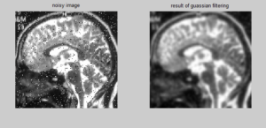
Removal of Noise & Smoothing

Besides diffusion, Gaussian filtering is also used for noise removal and smoothing of an image. It is usually carried out as a first step before applying any algorithm. The reason is simple: averaging causes random noise to get eliminated significantly and also lead to removal of discontinuities.

That’s all in this post where we’ve gone through Matlab implementation of isotropic diffusion, followed by pre-processing to be done on an image to get better result. We’ve also seen a number of test examples and how to choose the parameters of a Gaussian filter.

If you’ve any query, suggestion or feedback on the topic, then please leave a reply below. I will be more than happy to answer your questions. You can also visit my Computer Vision page to go through all articles on the subject.

If the article has helped you in some way or other, then you can donate in order to support the website. Have a nice day!